How TabPFN Helps with Robust Planning Use Cases at tulanā

A central challenge faced by businesses in supply chain is that the future is uncertain. When making planning decisions, they have to make an assumption about future demand, and the resulting decisions can come with huge associated costs. For example, if the decision is how much inventory to stock without knowing future demand, then having excess stock could cost millions in tied capital, whereas not having enough stock could cost millions in lost sales. Having good demand forecasts is thus essential to making good decisions.

However, a demand forecast is not a decision by itself. Predicting the exact demand on a future date is not realistic, and in reality even the best forecasts will have some margin of error. So how do you make decisions knowing that your demand is always going to be uncertain? For example, how much stock should you order knowing that the demand might be somewhere between 50-150 units? Is it better to over-order or under-order? This is where decision intelligence comes in. Decision intelligence is the approach of using data, mathematical methods, and domain knowledge to inform good decisions. Specifically, decision intelligence is the complete lifecycle from building the forecasts to converting them to actual decisions.

At tulanā, our decision intelligence relies on probabilistic forecasts. As opposed to a deterministic forecast that predicts point values, a probabilistic forecast instead predicts a probability distribution which gives a range of possible values. This way, our decision models are able to take into account a range of possible scenarios, thereby producing decisions that are more robust to uncertainty.

Building a good probabilistic forecast, however, is a non-trivial step. There are a range of statistical and machine learning methods available for this, but the main challenge lies in the fact that real data can be messy, unclean, and sparse, and a good forecast could take significant development effort to build and maintain. This can increase the time-to-value for crucial decisions. Today there are also foundational models like TabPFN that can give well-calibrated predictions on real structured data sets without the need for data pre-processing or training.

In this blog, we investigate the impact of different forecasting strategies through a demonstration of our decision intelligence pipeline on a real robust planning use case.

Robust planning use case

Consider a pharmaceutical company that produces a specialty life-saving drug for a small population of patients with a chronic condition. Every week, their planners need to decide how much stock to order. But specialty drug production typically comes with long lead times and uncertain demand, so they cannot react on a week-by-week basis and need to instead plan in advance.

Such businesses operate under high risk and are allowed only small margins of error. This is because they have very high service level targets, since a stock-out means a patient goes without a life-saving drug. But such drugs also typically have high holding costs due to factors like strict storage and compliance requirements and expiration risks. This means that both over-stocking and under-stocking can be very costly. Given these risks, the planners need to decide on a re-order policy: i.e., on any given week, should they order more stock? And how much?

This is a real robust planning use case faced by one of our customers. For this demo, we generate synthetic demand data so that it closely resembles the customer data. (See figure)

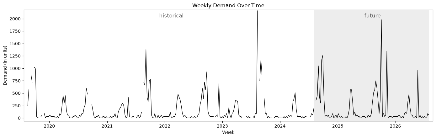
In this scenario, we have weekly demand over a seven-year period. We will treat the first five years as historic demand, which we will use to build our forecasts and choose a good re-order policy. The last two years will be treated as future demand, which we will use to evaluate the forecasts and the policy.

What makes this demand data challenging:

• The demand is steady for a majority of the weeks, but there are seasonal heavy-tail surges: think of patients that are on a steady dose all year round, but seasonal surges cause demand to spike at specific times of the year. And in particularly bad years, the seasonal surge could be unusually extreme.
• The demand data is unclean: here we synthetically added missing demand to make it unclean. In real life, this can happen for a variety of reasons, such as the demand data not being logged correctly or an issue with the underlying ERP system resulting in data corruption.

The goal is to derive a good re-order policy that can meet service levels at a high rate while minimizing storage costs. Our approach here will be to:

1. Build a good probabilistic forecast for future demand
2. Using the forecast, run simulations against many possible futures to find a re-order policy that best balances service levels against storage costs

Building probabilistic forecasts

Building a probabilistic forecast is about answering the question: knowing historic demand, what can we say about the future demand distribution?

1. Empirical estimation

The most straight-forward way of doing this is to just use the historical demand distribution to estimate future demand distribution. That is, we just compute the 5th, 10th, 25th, 50th, 75th, 90th, 95th percentile of demand over the entire history, and assume that 5th, … 95th will be the percentiles of demand in the future as well.

The figure below shows how this distribution fits on the actual future demand.

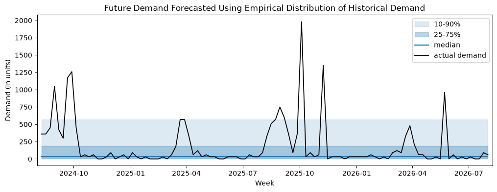
While simple, the empirical distribution does say something meaningful about demand. For example, the 90th percentile of historic demand is 570 units. If the pharma company maintained a stock of 570 units every week, then they would be able to serve 92% of future demand.

2. A simple linear model

From the chart we see that the empirical distribution does not capture any seasonality. It assumes that the demand distribution is the same all throughout the year. But there are a variety of statistical and machine learning methods for probabilistic forecasting that can better capture patterns in the data.

Let’s build a forecast using a simple linear model:

• Data pre-processing: data quality is very important for any ML model. Since our demand data contains missing values, we will need to use some imputation strategy to fix this in a pre-processing step. Here we do this by just interpolating demand on missing weeks using demand in the neighboring weeks.
• Feature engineering: we create 9 calendar features that are classic when it comes to time series data:
  • Week of year: Captures the absolute position of the week in the year
  • Eight harmonic features:  To capture seasonality, the model would need to know where in the year the week sits. But just using “week of year” is not sufficient. To the model, a plain number is just a position on a number line, so it would treat week 51 (late December) as being as far as possible from week 0 (early January). So we introduce harmonic features: sine and cosine functions of week of year. These transform week of year into a circle where week 51 will sit right next to week 0. If we just used a single sine and cosine function, then it won’t be able to capture sharp peaks. Using multiple functions helps capture the bends more sharply (using too many can cause over-fitting). So we use eight harmonic features (see code snippet below).
• Model: We used sklearn’s linear_model.QuantileRegressor . To learn the distribution, we fit 9 different models for 9 different quantile values: q=0.01,0.05,0.1, 0.25,0.5,0.75,0.9,0.95,0.99.

# Eight harmonic features:
# sin(2nπw/52), cos(2nπw/52) where w is week of year and n=1,2,3,4

sine_features = [
	sin(2*n*pi*week) for week in range(52)
	for n in range(1,5)
]

cosine_features = [
	cos(2*n*pi*week) for week in range(52)
	for n in range(1,5)
]

‍


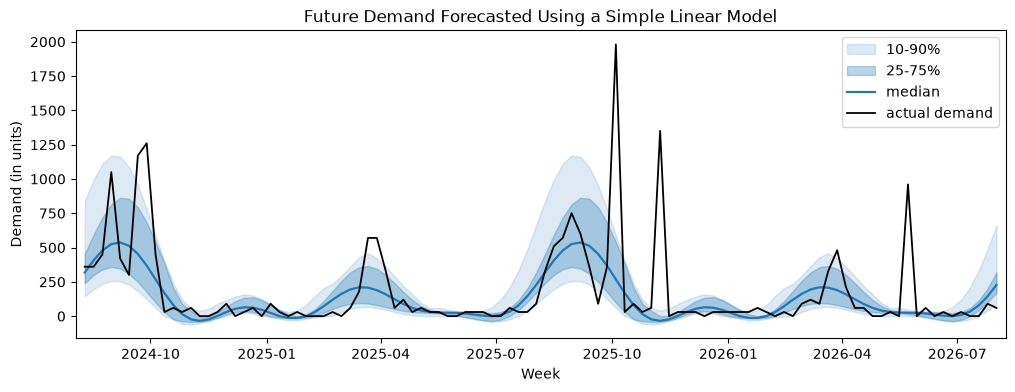
From the chart below, we see that a basic linear model with the right features already fits better than the empirical distribution. In periods of low demand, the distribution bands are much narrower and fit the demand more closely, and in periods of high demand the distribution bands are broader and are able to capture some of the seasonal surges.

3. A tuned ensemble model

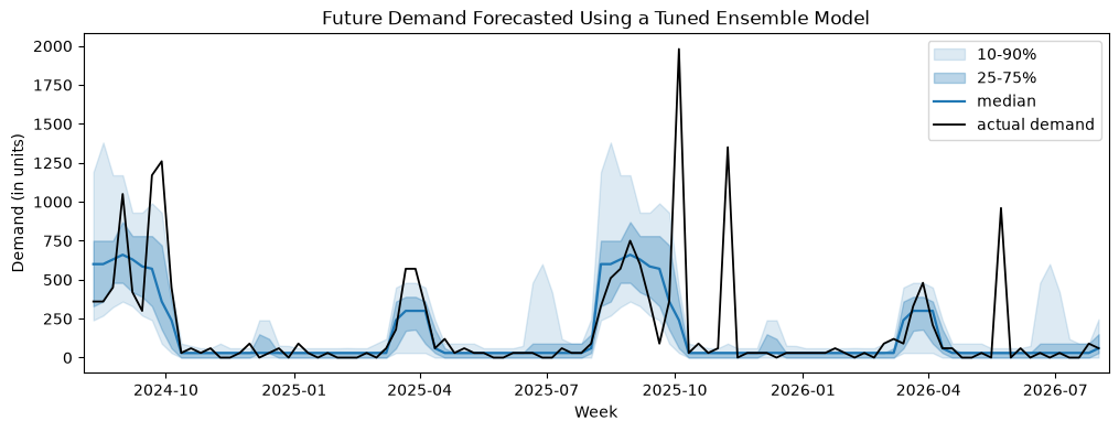
Our simple linear model captures seasonality, but it does not capture the sharpness of the surges. A linear model combined with the sine and cosine features results in smooth seasonal curves where the surges are much more spread out. But the seasonal surges in the actual demand data are much more sudden and narrow. The simple linear model is quite basic and spending more development effort into building a more sophisticated model could result in a better fitted forecast.

A popular ML model for probabilistic forecasting is Quantile Regression Forest which is an ensemble model that, instead of predicting single point values, predicts a range of quantiles. Such ensemble models are also able to fit much better around sharp edges. But they are prone to over-fitting and need to be tuned.

Let’s build our ensemble model with hyper-parameter tuning:

• Data pre-processing: we use the same pre-processing approach as before (imputing missing demand values by interpolating demand from neighboring weeks)
• Feature engineering: we use the same calendar features as before (week of year + the eight harmonic features)
• Model: we use Quantile Regression Forests which predict a range of quantile values (as opposed to needing to fit a separate model for each quantile, like we did for the linear model). We use the following maintained implementation: https://zillow.github.io/quantile-forest/
• Hyper-parameter tuning: since random forests are prone to over-fitting, we perform hyper-parameter tuning. We tune the tree depth and leaf size with rolling origin cross-validation over the history (training on earlier weeks, validating on weeks one year ahead, and then sliding the window)

From the chart below, we see that this model captures the sharp seasonal surges much better than the simple linear model.

4. Using TabPFN

One drawback of ML models when it comes to forecasting is that they rely heavily on input data. This is fine when the data is clean and large enough for the models to learn patterns in the data. But as the data sets get more challenging, ML models require increasingly more effort in terms of feature engineering, model selection, model training, and hyper-parameter tuning to produce good forecasts.

There are now foundational models that perform predictions on tabular data. A popular model is TabPFN. Foundational models like TabPFN are already pre-trained on large amounts of tabular data, so they don’t need to be re-trained. That is, they can spot causal relations in the data without needing to be trained on it. Because of this, they can perform better on challenging data sets as compared to ML with less development effort.

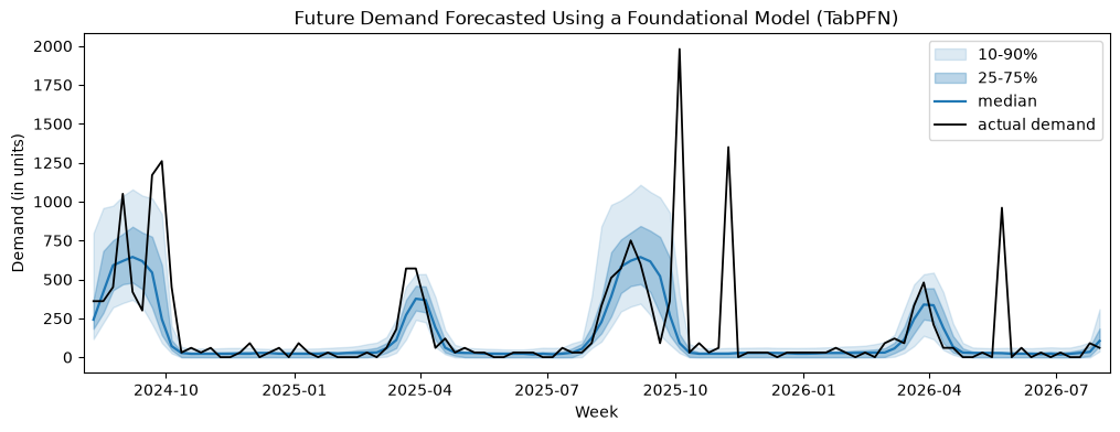
We use TabPFN’s time series package https://github.com/PriorLabs/tabpfn-time-series. Unlike for the ML models, we don’t need to do data pre-processing, feature engineering, or hyper-parameter tuning. We feed in the historical demand and TabPFN returns a stochastic forecast for future demand.

Looking at the chart below, we see that it is able to produce a good fit on future demand without any development effort. (Note: this was built using TabPFN-3, which was the latest version at the time of writing this blog.)

Comparing the forecasts

So far we’ve been commenting on the accuracy of the forecasts based on what the charts above look like. A more quantitative way of doing it is to use a metric like Continuous Ranked Probability Score (CRPS). Since we don’t forecast point-values, we can’t use metrics like Mean Absolute Error (MAE) or Mean Absolute Percentage Error (MAPE). CRPS is a generalization of MAE to probability distributions.

Intuitively, CRPS rewards the forecast distribution for putting probability mass close to the true demand and penalizes when either the probability mass is away from the true demand or if it’s too wide and spread out. The lower the CRPS, the better the forecast. A CRPS of 0 means that the forecast is perfect, i.e. it places all the probability exactly on the true demand.

The table below shows CRPS of the different forecasting methods. We see that TabPFN fits the true demand the best, followed by the tuned ensemble model, followed by the simple linear model, with empirical estimation performing the worst.

Deriving re-order policies using the forecast

A stochastic forecast tells us the possible range over which future demand can fluctuate. Knowing this, we can make intelligent decisions about when to order stock and how much. These decisions (known as re-order policies) can then be optimized to have the lowest total costs over the entire time horizon.

For specialty pharmaceutical drugs, these costs typically run high. We make the following cost assumptions in this demo:

‍

There are many ways to find good re-order policies. In this demo, we are going to be running Monte Carlo simulations by sampling different demand realities from a probabilistic forecast and compute the total average cost. We are going to perform this for a range of different re-order policies and derive one that has the least average cost over several simulation trials.

The better the forecast, the closer the sampled realities will be to the true demand, and the more likely the derived policy is to minimize the total cost on the actual future. To show the impact the forecast quality can have on reducing the total costs, we will repeat the above using the four different forecasts that we developed in the previous section.

Assumptions

Lead time: To keep things simple, we are going to assume a constant lead time of 6 weeks. This means that any order placed today arrives 6 weeks later. This makes having a good forecast important, because if a surge is coming in 6 weeks then it needs to be planned for today.

Starting stock: The simulations are being played out over two years of future. Assuming 0 units of starting stock would not be realistic and would result in heavy stock-outs over the first six weeks (since any order will take six weeks to arrive). Instead we make the reasonable assumption that they are adequately stocked to meet demand at a high service level of 98% over the next six weeks of lead time. So we set the starting stock as 4525 units, which is the 98th percentile of historical lead time demand.

Re-order policies

There are many different types of re-order policies. For this article, we will restrict ourselves to the standard (s, S) re-order policies (whenever the stock falls below s units, order up to S units). s is called the re-order point. Given that the lead time is six weeks, s should be chosen such that on-hand stock is always sufficient to meet demand at a certain service level q over the next six weeks. For a given q:

• s is chosen as the qᵗʰ percentile of lead time demand, which is derived from the demand forecast distribution.
• and S = s + Q, where Q is the classic Economic Order Quantity (EOQ) determined by ordering cost K, weekly holding cost h, and average weekly demand D. (See here)

Simulations

For a single choice of q, our re-order policy is fixed (as defined above). But how do we choose a good q? If chosen too small, we run the risk of not having enough stock for the upcoming 6 weeks. And if chosen too large, we end up paying more in storage costs than necessary.

Since we have an estimation of future demand from our stochastic forecasts, one approach would be to evaluate different choices of q using Monte Carlo simulations. A single Monte Carlo trial runs like this:

• Draw one possible future: we sample a demand value for every week over the two-year horizon from the forecast distribution.
• Play out the chosen policy week-by-week: starting from our starting stock, we step through each week, receive any order that arrives (placed six weeks earlier, due to the lead time), serve that week’s demand from stock (any demand we can’t meet becomes a lost sale), and then apply the (s, S) rule to decide whether to place a new order.
• Tally the cost: we add up the total cost incurred every week (holding + order + COGS + lost sales) and get a total over this sampled future.

We run N trials* and compute the expected total cost over all the trials. Since each trial samples one future demand scenario and we perform several trials, we are selecting for a re-order policy that has the least expected cost over a range of future demand scenarios.

* N is chosen large enough to ensure separation of estimated total costs for different policies and forecast methods with 95% confidence.

Comparing the outcome of the different forecasting strategies

When choosing the best re-order policy, our simulations are not using any information about the true future demand (because in real use cases this information is not available beforehand). Instead, they are sampling futures from a probabilistic forecast. In the previous section, we built four forecasts using four different strategies and the CRPS score showed us the differences in accuracy between them. But what does this difference mean for the actual outcome?

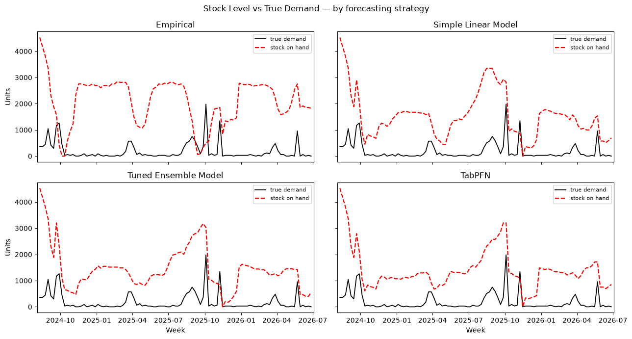
For each of the four forecasting strategies, we run our simulations using the respective forecast and choose the best re-order policy. We then play out this re-order policy week-by-week against the actual future. That is, instead of sampling a future demand scenario from a distribution like we did in the simulations, we use true demand to update the on-hand stock and compute total costs. We then measure the total fill rate over the future (total percentage of demand served) and the total costs.

‍

The results show us the importance of an accurate forecast on the re-ordering decisions:

• The demand forecast from the empirical estimation strategy had the highest CRPS score, and that from TabPFN had the lowest CRPS score. Looking at the total costs, we see that the re-ordering policy derived from TabPFN forecasts results in ~$50M lower total costs when compared to that derived from empirical estimation.
• The re-order policy derived from empirical estimation has the lowest fill rate (highest lost sales) and the highest holding costs. This is because the forecast does not capture the peaks and the dips in the demand, which results in high holding costs as well as high lost sales. For example, not seeing a demand surge coming and only reacting once the surge has depleted on-hand stock, resulting in higher lost sales. (see chart below)
• We also see benefits of a better fitted forecast when we compare the results of the policies between the two ML forecasting strategies. The policy derived from the forecasts of the simple linear model results in a higher fill rate when compared to that derived from the forecasts of the more sophisticated tuned ensemble model, despite the former having a worse forecast fit. This is because the resulting distribution bands for the simple linear model are broader which makes the policy hold more stock than necessary. This results in higher holding costs, which causes the total costs of the simple linear model policy to be ~$2M higher than that due to the tuned ensemble model policy. (see chart below)
• Lastly, the re-order policy derived from TabPFN results in highest fill rate as well as the lowest holding costs, with total costs that are ~$4M less than that of next best policy (one derived from the tuned ensemble model). As we can see in the chart below, a better-calibrated fit results in lower stock during periods of low demand and in sufficiently high stocks in periods of surges.

Conclusion

When it comes to planning decisions with high associated costs and risks, the role of decision intelligence becomes very important. Use cases like that of the pharmaceutical company in our demo are very common in the real world, and it’s something that we constantly solve for at tulanā. The individual components of the decision intelligence pipeline like the forecasts can massively affect the final outcome. This makes building forecasts an important first step of solving such planning problems.

But this takes time investment. At tulanā, we very commonly use ML methods for this, which comes with development effort. As we saw in this article, there is a whole lifecycle involved: data pre-processing, feature engineering, model selection, hyper-parameter tuning. Something that we didn’t explore here, but is another real challenge is that of updating the forecasts when the data drifts. On the other side, a simple procedure, like empirical estimation, is both easy to build and update. But, this often results in poorer decisions resulting from inaccurate forecasts. So the development effort is worth the time investment, but it does increase the time-to-value of the resulting decisions.

Today there are foundational models, like TabPFN, that come pre-trained and don’t require the ML lifecycle to produce a well-calibrated forecast. Because they can just be “plugged in” to the decision intelligence pipeline, they also don’t need maintenance in instances of data drifts. For our robust planning use cases (like that of the pharmaceutical company), this to us is an exciting possibility.

Planning decisions (like the one in the demo) have to be made in advance under uncertainty, and once made they cannot easily be taken back. The costs of getting them wrong are high on both sides: excess stock ties up capital, while a stock-out for a life-saving drug means a patient goes without. The same holds for planning problems well beyond pharmaceuticals, from crew planning at an airline to maintaining critical infrastructure, and each comes with its own risks. Decisions with this much at stake should not rest on a best guess. This is where decision intelligence comes in, and it is what we build at tulanā.

‍